The Variance of Yotta Savings Accounts
My girlfriend recently got a Yotta savings account which has an interesting twist: instead of paying interest like a normal bank, they buy you lottery tickets. This makes saving more exciting, since you have a small chance of winning millions of dollars.
Now, my first thought was that this must be a terrible deal for whoever’s playing, since the lottery is generally considered a bad investment. But it turns out the Yotta lottery actually has pretty good odds. People have calculated the average return to be around 2.6% APY1, which is not a bad return for a savings account. This will likely decrease as they become more established and get more users.
What is the variance of Yotta interest?
One question I haven’t seen answered on the internet is about the variance of the APY. Sure, maybe the average investor gets 2.6% APY. But that might mean most people get 0% and one person wins a few million dollars. If I’m going to invest, I’d like some guarantees on the lower-bound of the amount of money I’m going to get back.
This is a really straight-forward instance of the law of large numbers: the more tickets you buy, the closer you’ll get to the average return. But before we break out the math, let’s start with some simulations to get some intuition of what to expect.
Let’s suppose 10k people each invest $10k in a Yotta savings account. How much interest will each of them earn? We can simulate this scenario with a pretty simple python script:
- $10k buys each person 400 lottery tickets per week.
- We can simulate the lottery drawings with a random number generator to predict how much money2 each person will win from their 400 tickets. (No split prizes.1)
- Rinse and repeat for 52 weeks, keeping track of the total money won for each person.3
The results are plotted in the histogram below. On the x-axis is an amount of money, and the y-axis shows how many people won that much money via lottery tickets.
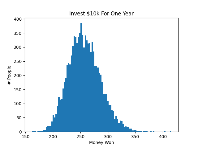
As expected, the average money won is around $260 (2.6% APY). However, some people won as little as $200 (2.0% APY) and some as much as $350 (3.5% APY). No one won less than $150 (1.5% APY).
So the variance isn’t that bad. Of course, if you invest less money you get less tickets, and so the variance will increase. Below is the same experiment when people invest $1k each.
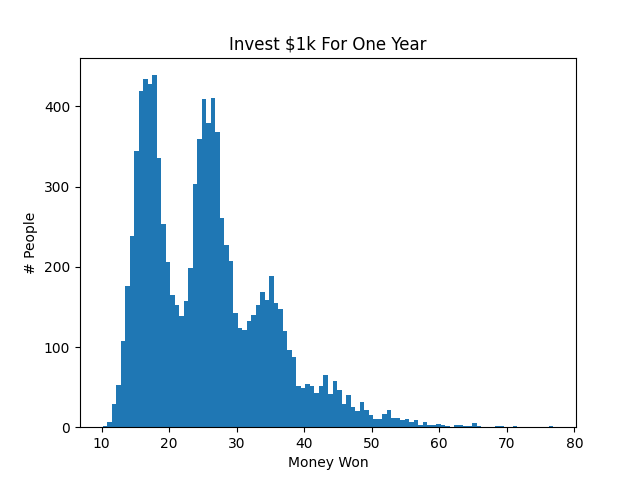
In this case, the average still seems to be around 2.6% APY. However, some people get back as little as 1.0% APY, and there’s a large skew right, with some people getting as much as 6.0% APY. If you’re interested in running more experiments, I’ve provided the python snippet below. (If that’s broken you can also grab the code on github.)
Tail Inequalities
I mentioned earlier that buying many lottery tickets is a very straight-forward instance of the law of large numbers: the more tickets you buy, the closer your winnings get to the expected APY. But what if I want to quantify exactly how far my earnings will be from the average? For example, if I invest $10k for one year, how likely is it that I earn less than $200?
This is exactly the question that tail inequalities answer. Suppose I have a random variable \(X\). Tail inequalities tell us how probable it is that \(X < t\), for some value of \(t\). There are several types of tail-inequalities you can use, depending on how much information you have about \(X\):
-
The Markov Inequality is the simplest version, which you can use if you only know the expected value of \(X\).
-
The Chebyshev Inequality is more complicated, taking into account both the expected value of \(X\) and its variance.
-
Chernoff Bounds usually give you the tightest bounds, but are only applicable when \(X\) is a sum of multiple independent random variables.
Technically we could apply Chernoff bounds, since the amount that we win in a year is the sum of the amount that we win for every ticket we buy that year. But that requires a little more elbow grease than I’m willing to put in at the moment, so we’ll just use Chebyshev bounds. Here’s the theorem:
Theorem (Chebyshev’s Inequality) Let \(X\) be a random variable with expectation \(\mu_X\) and standard deviation \(\sigma_X\). Then for any \(t \in \mathbb{R}^+\),
\[Pr[|X - \mu_X| \leq t \sigma_X] \leq \frac{1}{t^2}\]Let’s break this down for our case:
| Math stuff | Our case |
| \(X\) | The amount of money we’ll earn if we invest $10k in a Yotta savings account over one year. |
| \(\mu_X\) | The average value of X. ($260) |
| \(\sigma_X\) | The standard deviation of X. ($29)4 |
| \(Pr[|X - \mu_X| \leq t \sigma_X]\) | The probability that the money we earn is \(t\) standard deviations away from the mean. |
So let’s say we want to know the probability that we earn less than $200 in a year. That’s more than two standard deviations away from the mean. The Chebyshev theorem tells us that the probability that we make less than two standard deviations below the mean is \(\frac{1}{2^2} = 1/4\).
So Chebyshev guarantees that we’ll make more than $200 with at least 75% certainty. But remember, that’s just a bound. Based on our simulations, the probability that we make more than $200 is likely much higher than 75%. I would probably say it’s around 95% based on the histogram.
Central Limit Theorem
Now, you might have noticed that our first histogram looks essentially like a normal distribution. This happens all the time and is the subject of the central limit theorem (CLT). The CLT says that if you buy enough lottery tickets, the amount of money you make that year will fall on an approximately normal distribution. The mean of this normal distribution is the sum of the average value of a ticket, while the variance is the sum of the variance of each ticket.
If we can verify that the distribution is approximately normal, as we have above with the $10k scenario, we can skip calculating the Chebyshev or Chernoff bounds and just assume the distribution is normal. Plugging in the average and standard deviation into this normal distribution calculator tells us the probability of making more than $200 is 98%. This is much more in line with the results of our experiments, if slightly more hand-wavy.
You have to be careful with this approach, however, since not all distributions will be normal. For example, the second scenario we tested, where each person invested $1k, showed that the distribution wasn’t very close to a normal distribution. In that case, it might be better to apply Chernoff or Chebyshev bounds.
-
Some prizes can be split between multiple winners (such as the $10M prize). If more people are playing, then split prizes get smaller. Since we’re interested in the “worst-case” scenario, we assume the actual payout for all split prizes is $0. In this case, the average APY is 2.6%. ↩ ↩2
-
We used the payouts from this spreadsheet. ↩
-
For simplicity, we did not compound the weekly interest. This can be changed in the python snippet, if you care, but it does not impact growth too much. ↩
-
The variance of a single ticket is roughly 4 cents. The variance of a sum of independent random variables is the sum of their variances. So for 400 * 52 = 20,800 tickets, the variance is about $842. The standard deviation is the square root of the variance. ↩